UAV Towed Sensor
Designed and flight tested a deployable sensor for the special mission requirement.
By Jonathan Lee.
March 17, 2021

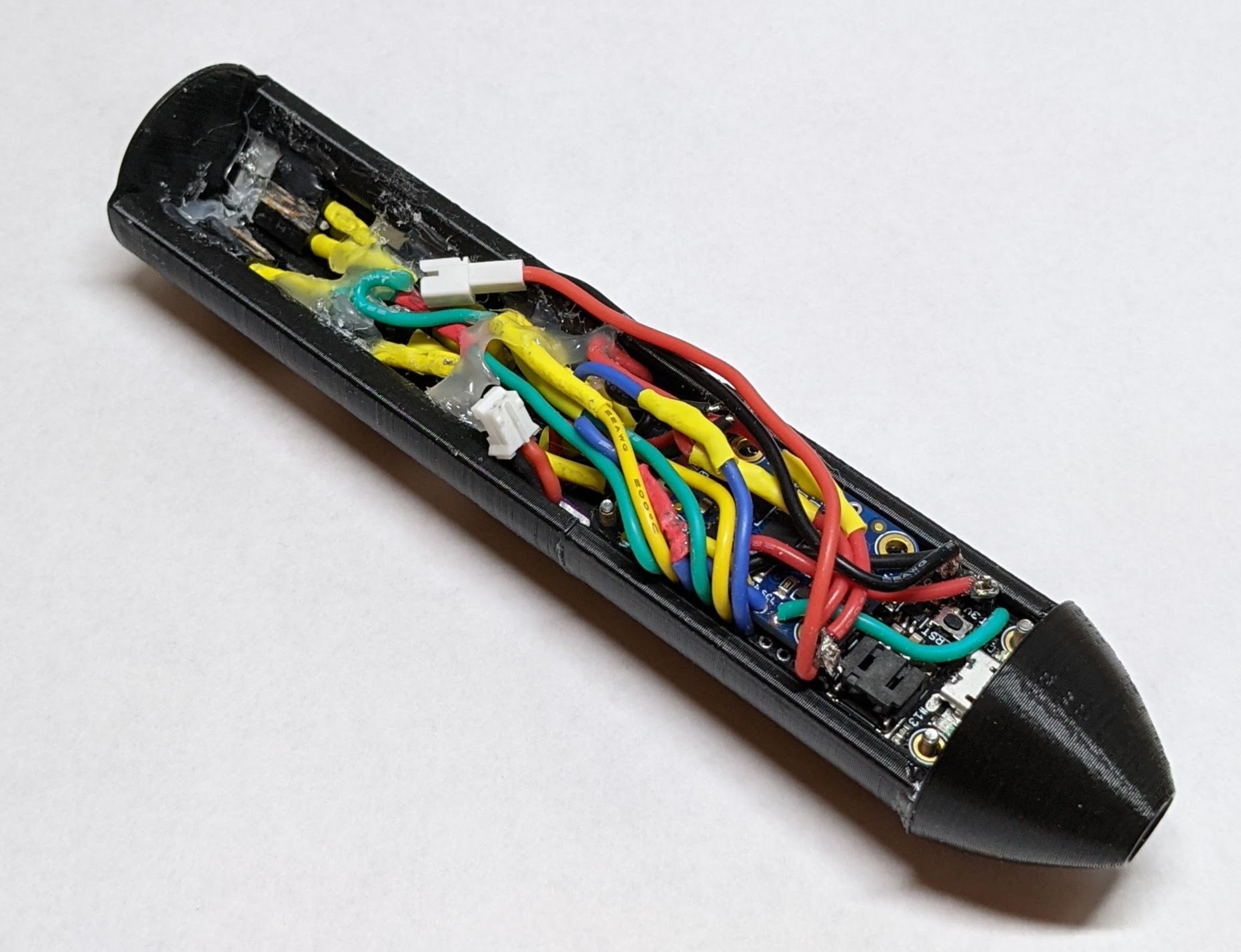
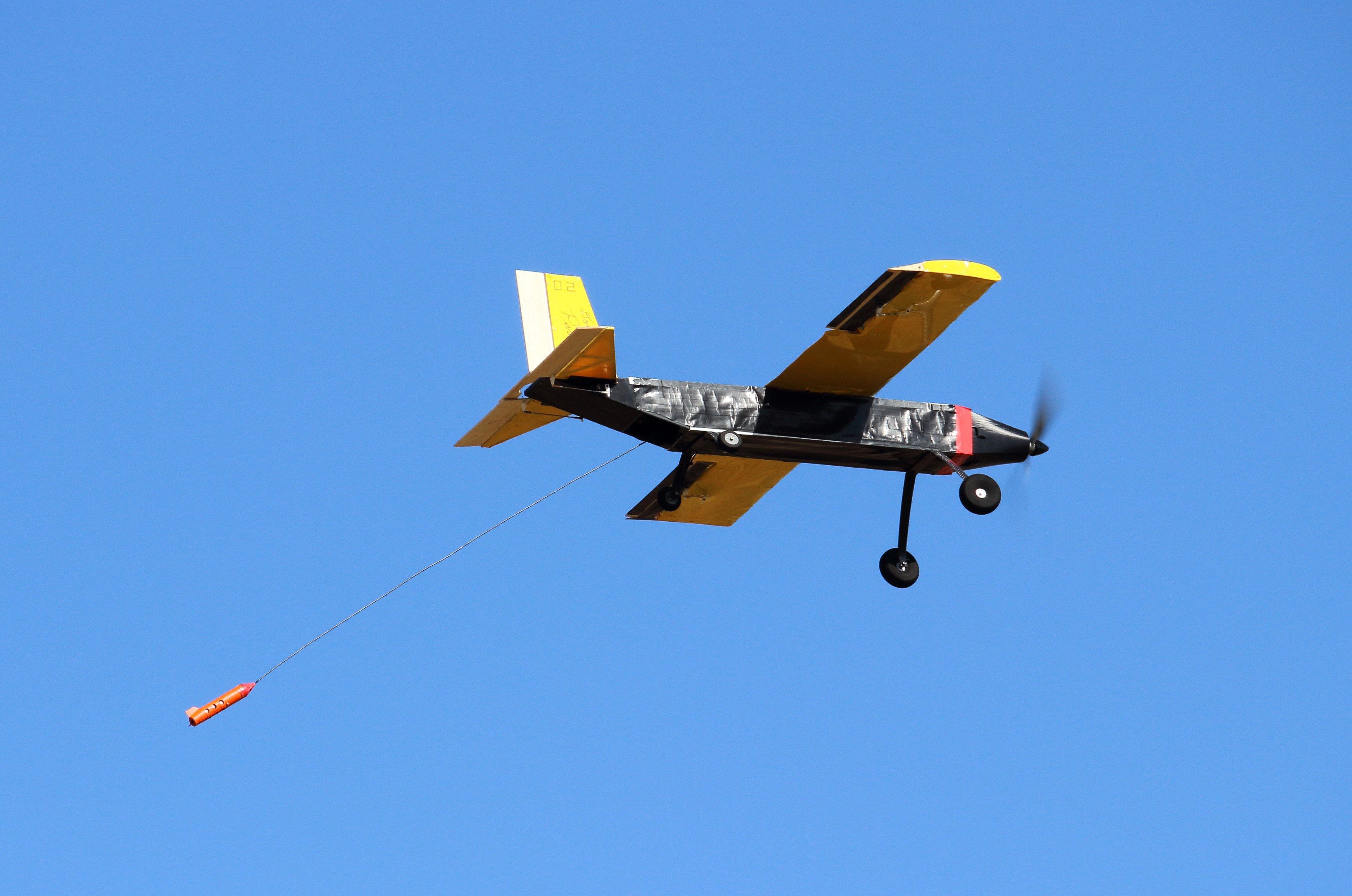
Table of Contents
- Table of Contents
- Overview
- Design Philosophy
- Conceptual Design
- Preliminary Design
- Detailed Design
- Performance Testing
- Performance Results
- What I Learned
Overview
This post is about the cable-towed sensor I designed for the GW Design/Build/Fly (DBF) team. The American Institute of Aeronautics and Astronautics (AIAA) DBF competition challenges engineering students from around the world to develop the best electric powered, radio-controlled aircraft to suit a special mission. The mission component changes every year and is inspired by a real-world aerospace application. The UAV towed sensor was the special mission component for the 2021 competition. UAV towed sensors have a variety of practical applications. For example, the AirBIRD is a commercial sensor used to conduct magnetometer surveys from autonomous drones. And the AN/ALE 55 is a fiber-optic towed decoy designed to protect fighter jets from incoming missiles.
The sensor we were required to build is an aerodynamic pod capable of (1) deploying from the airplane fuselage in midflight, (2) exhibiting aerodynamic stability during operation, and (3) returning to its storage position before landing. The sensor also required at least 3 bright navigation lights to be visible from the ground and controlled by wire. As an additional feature, I also decided to equip the sensor with a 9-axis Inertial Measurement Unit (IMU) to capture flight data to a microSD card. The data is processed post-flight and is used to determine sensor flight characteristics and improve sensor design. The sensor design followed the standard aircraft design process steps of conceptual, preliminary, and detailed design. The formal design process is detailed in the 2021 GW DBF Design Report.
2021 was a milestone year for the GW DBF team. We achieved our first flight in the club’s 5 year history and successfully completed mission testing for our design. The airplane and sensor performance exceeded our expectations with the consistent execution of sensor deployment, retrieval, stability, and lights functioning flawlessly. The team’s success was an impressive feat considering the unique circumstances of virtually and remote work for the majority of the year. The aircraft design started in September 2020 and performance testing concluded in March 2021. Here is a highlight video of our test flights during spring break:
Design Philosophy
Creating a good final product involves iteration because the first prototype is never perfect. But since time is limited, creating many design iterations becomes inefficient. A good strategy is to create a batch of designs that can be tested and evaluated in parallel. Then, like a genetic algorithm, select the best design and evolve it for the next iteration. This strategy leads to rapid design evolution in less time. I achieved this goal by using these putting an emphasis on:
- 3D printing and rapid prototyping
- Modular and interchangeable parts
- Repeatable and controlled testing
- Sensor data and performance evaluation
Conceptual Design
During the conceptual design phase, the mission requirements and constraints were detailed. New ideas were brainstormed and existing solutions were reviewed. A design candidate was selected for the preliminary design phase.
Mission Requirements
The aircraft must be equipped with a sensor to satisfy mission objectives. The sensor must be cylindrical in shape, with a minimum diameter of 1.00 inch and a minimum length to diameter ratio of 4. For the cargo transport mission, sensors must be transported inside shipping containers in the fuselage of the plane. The goal is to transport as many sensors as possible for the longest flight duration possible. For the deployment mission, the sensor must be deployed on a tow cable 10 times the length of the sensor. The sensor must be aerodynamically stable during deployment, operation and recovery. Additionally, the sensor must have a minimum of 3 external lights that can be viewed while in flight. The lights must blink in sequence and be controlled via the transmitter with its own battery power supply.
Literature Review - Stabilizer Fins
To prevent the sensor from rolling and spinning, some sort of stabilizer might be necessary.
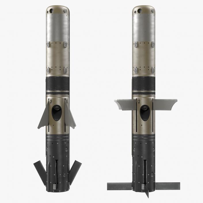
There are many stabilizer designs for cylindrical flying objects. Missiles and rockets have very similar constraints to our requirements – stable in flight with a low aspect ratio. Many designs have 4 control surfaces that provide either passive or active stabilization with a guidance control system. This fin configuration allows for pitch and yaw adjustments that keeps the missile pointed towards its target.
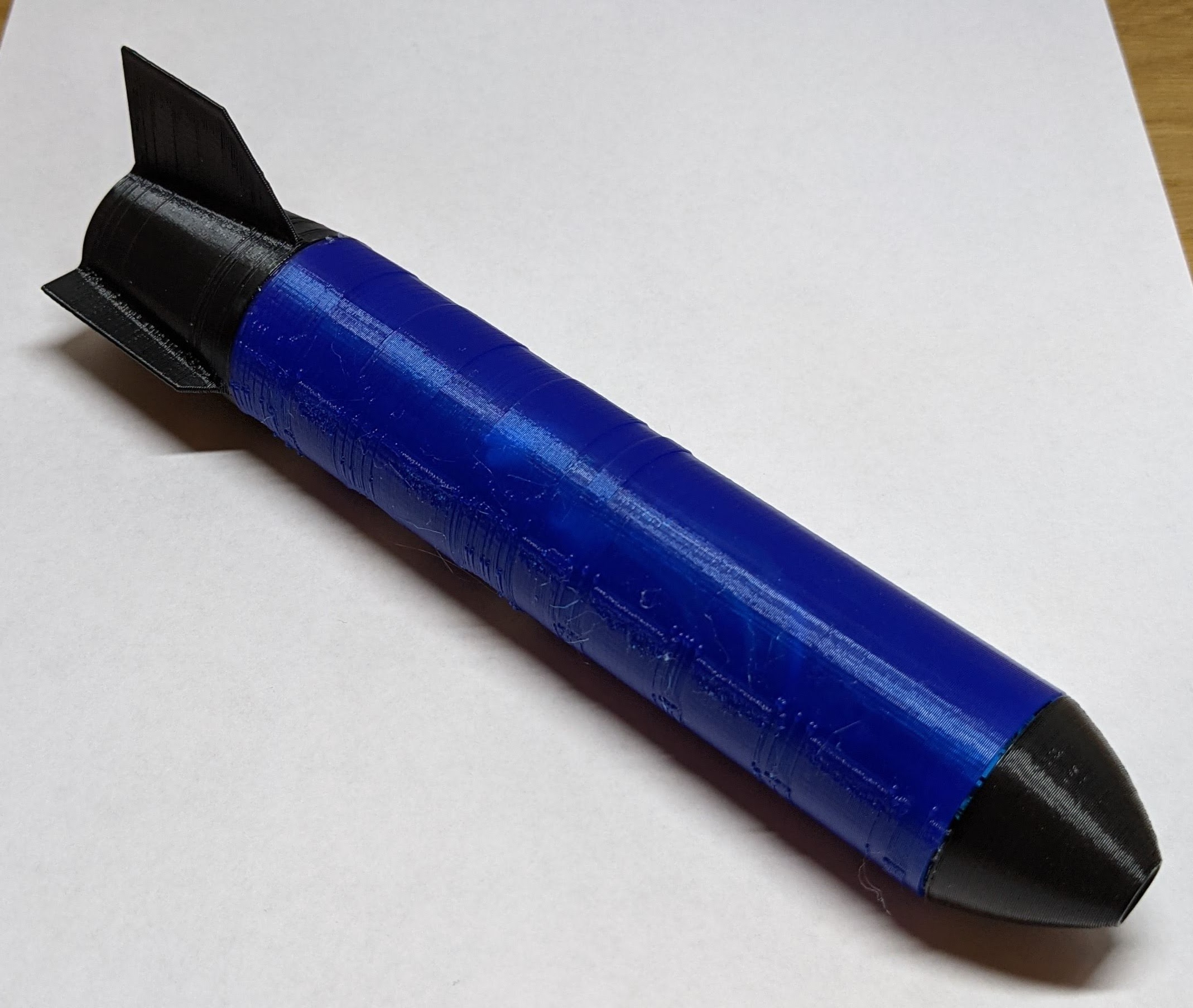
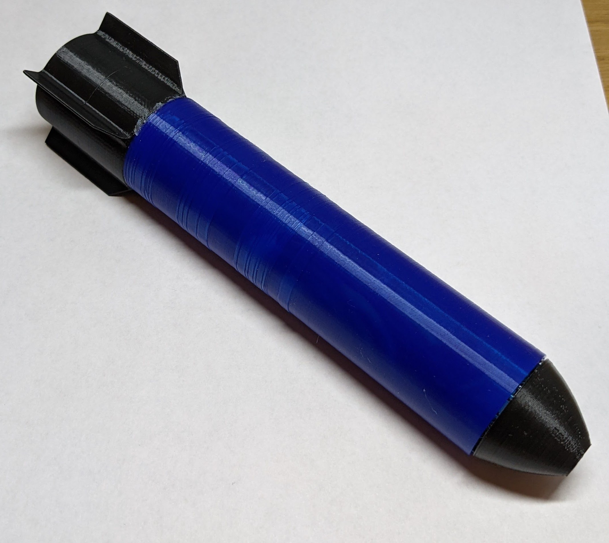
Another stabilizer design is a dihedral, which requires only two fins in a ‘V’ shape. The swept back fins create balancing drag forces that reduce the tendency for the sensor to spin. This configuration is used in sea sensor probes and SpaceX’s Starship prototypes. They can also be found in aircraft wing designs due to the inherent stability produced by the dihedral effect.
An early design concept used a dihedral design with deployable fins. The fins fold away for storage and deploy during flight. Each fin would be able to articulate and change its pitch via a small servo mounted inside the body. The fins could be actively controlled by a microcontroller and IMU to provide additional stability. This concept was eventually scraped because rules clarifications forbid active control and deployable fins.
Stabilizer Fin Decision Matrix
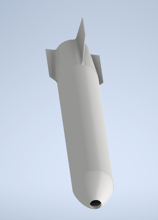
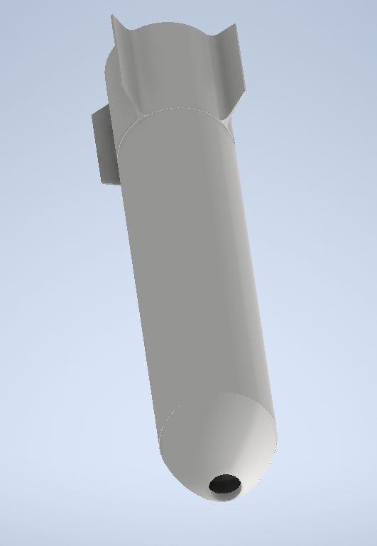
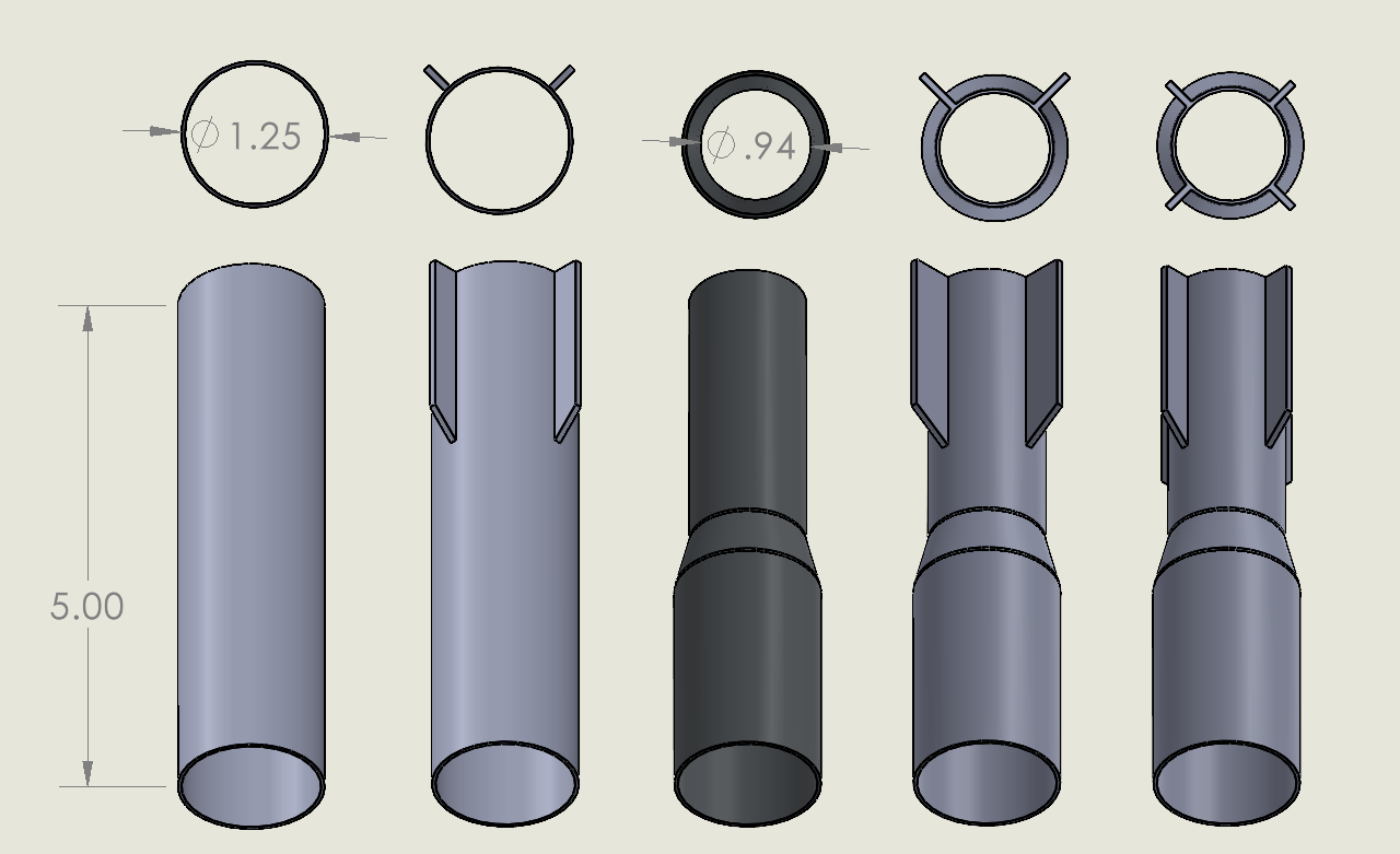
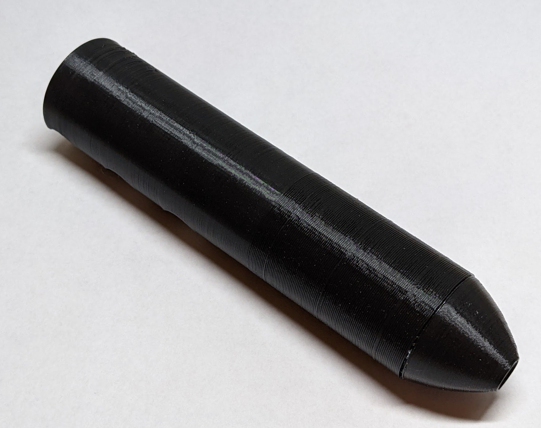
The main body of the sensor consisted of a cylinder with a nose cone. This would be the control shape. Then three stabilizer fin designs were considered: one with a large rudder, four fins in an “X” pattern, and a dihedral. The design of the sensor would be modular, to allow different fins to be easily be swapped out and tested.
All sensor fin designs were 3D printed and tested. The score of the sensor is based on the weighted sum of three criteria: aerodynamic stability, storage density, and drag. Having an aerodynamically stable sensor is the most significant criteria as it enables smooth deployment and retrieval, predictable flight characteristics, and more consistent external light visibility. A storage dense sensor is also important, as more sensors can be packed into the fuselage. Finally, low drag will equate to a higher top speed and lower lap times.
Below is the initial decision matrix with each of the designs. It is updated as each of the designs are tested and analyzed. The design with the highest score is selected.
| Criteria | Weight | Cylinder | Large Rudder | X Fins | Dihedral |
|---|---|---|---|---|---|
| Stability | 65% | TBD | TBD | TBD | TBD |
| Storage Density | 25% | 5 | 2 | 3 | 4 |
| Drag (low) | 10% | TBD | TBD | TBD | TBD |
| Weighted Score | TBD | TBD | TBD | TBD |
Preliminary Design
During the preliminary design, the design was further refined and analyzed. Trade studies were conducted on sensor size and weight. Predictions of sensor performance were also established to assess aircraft characteristics and mission capabilities.
Sizing Trade
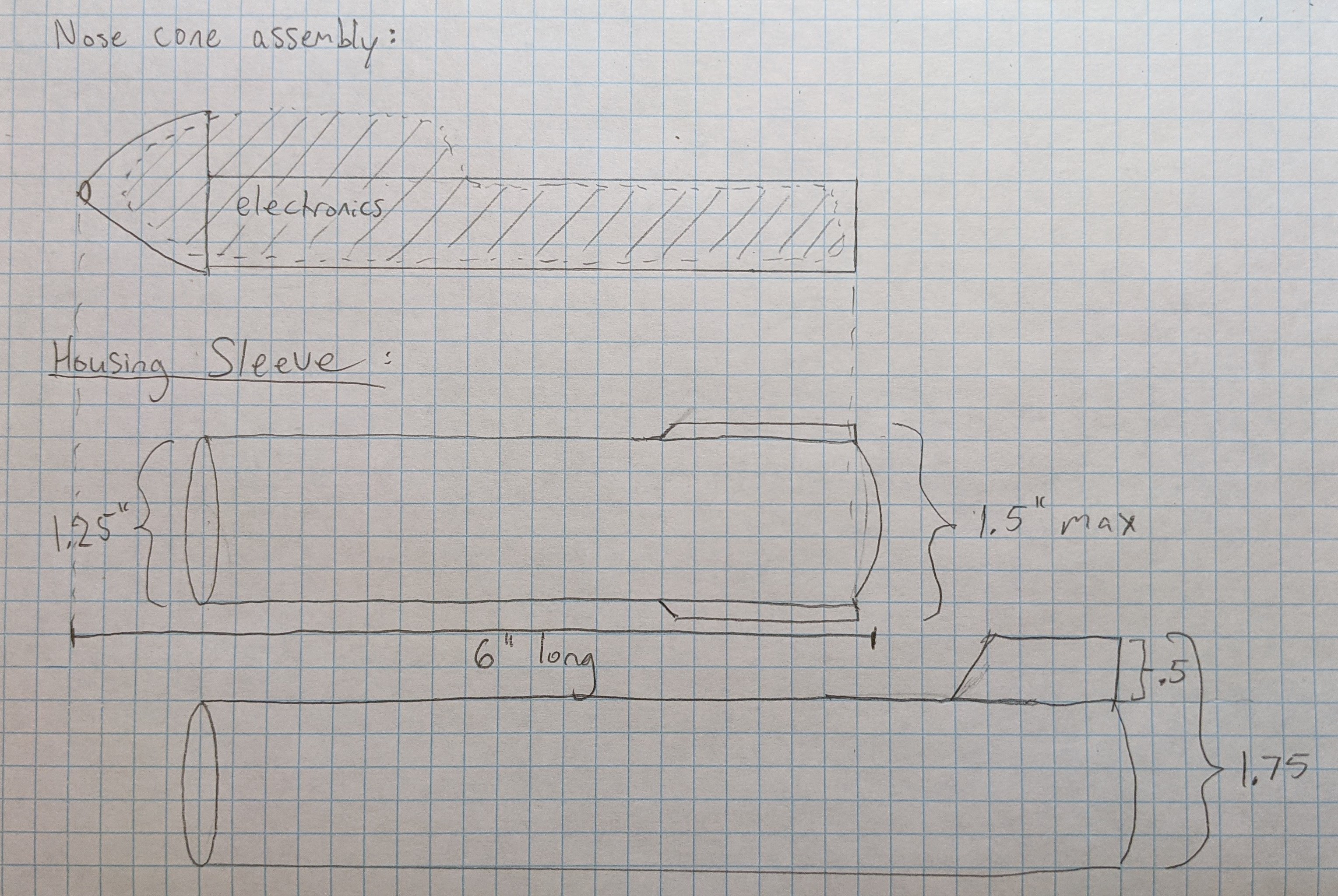
The sensor dimensions were selected based on mission requirement and physical limitations of the aircraft. The sensor’s internal electronics hardware necessitated a sensor diameter of at least 1.25”. Additionally, the minimum 1:4 length to diameter ratio requirement constrained the sensor to a length of at least 6”. While a longer sensor would directly increase the sensor mission score, it would also lower cargo storage capacity for the transport mission. Additionally, the tow cable length is directly proportional to the sensor length. Every additional inch of sensor length adds an additional 10” of tow cable. A longer sensor would add significant complexity to the deployment, towing, and retrieval of the sensor. Each of these factors translates to decreased mission reliability. As such, a minimal sensor length of 7.32” was selected to ensure all electronics could be housed inside, the nose cone could be attached, and tail fins could be added.
Weight Trade
The sensor weight also presented a trade off. Sensor weight is directly proportional to the Mission 3 score. However, it is also inversely related to the plane’s load capacity, thereby resulting in a lower Mission 2 score. A lighter sensor also improves aircraft flight characteristics, by reducing the center of gravity change during deployment and retrieval. The sensor weight was thus kept to a minimum weight of 0.3 lbs to improve flight dynamics and increase the likelihood of completing Mission 3 successfully.
Drag Analysis
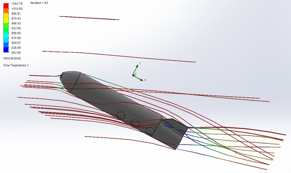
A comparison Computational Fluid Dynamics (CFD) analysis was performed to determine the drag caused by the sensor during towing. The results of the analysis provide an estimate of the drag produced. By knowing the coefficient of drag, the team can calculate the amount of drag from the sensor at any given speed the aircraft is going at. This helps determine the required plane configuration to account for this change.
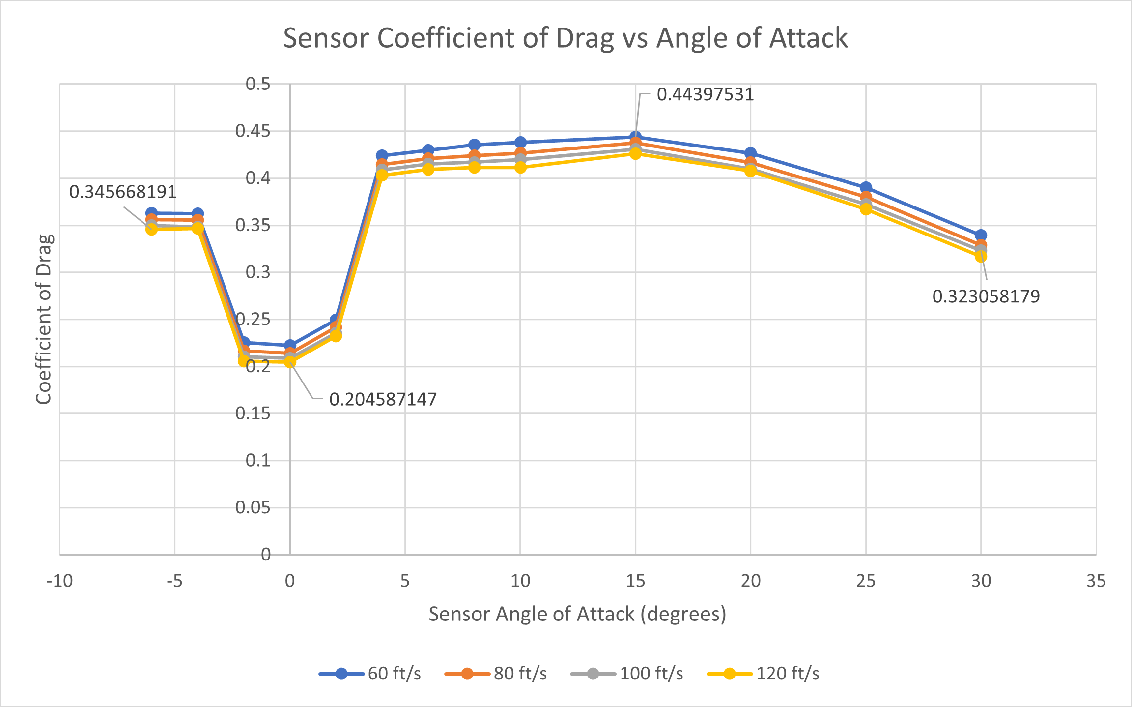
The plot above shows sensor coefficient of drag at various angles of attack and airspeeds. The coefficient of drag was calculated using the coefficient of drag equation, shown below, with data from the CFD analysis. \(C_D=\frac{2D}{\rho V ^2 A}\) The drag of the sensor was reduced at angles close to the horizontal. Higher airspeeds also reduce sensor drag. In ideal conditions between -2° to 2° of inclination and 120 ft/s, the sensor achieved an optimal coefficient of drag, \(C_D=0.205\).
Below is the \(C_D\) of the sensor with a dihedral fin design.
| 60 ft/s | 80 ft/s | 100 ft/s | 120 ft/s | |
|---|---|---|---|---|
| Cd_min @ 0° | 0.222 | 0.214 | 0.209 | 0.205 |
| Cd_max @ 15° | 0.444 | 0.437 | 0.431 | 0.426 |
The updated stabilizer fin decision matrix with drag scores:
| Criteria | Weight | Cylinder | Large Rudder | X fins | Dihedral |
|---|---|---|---|---|---|
| Stability | 65% | TBD | TBD | TBD | TBD |
| Storage Density | 25% | 5 | 2 | 3 | 4 |
| Drag (low) | 10% | 5 | 4 | 3 | 1 |
| Weighted Score | TBD | TBD | TBD | TBD |
Detailed Design
During the detailed design, the dimensional parameters, system architecture, and subsystem integration were all finalized. This included the electronics selection and schematic, CAD design, and controls implementation.
Electronics
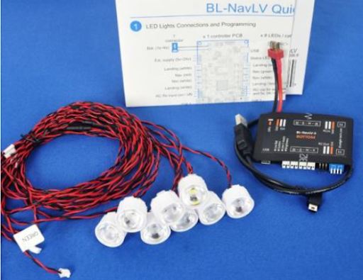
The sensor is required to have at least 3 flashing lights visible from the ground. Similar systems have been created for RC planes. The BL-NavLV is a navigation and landing system that can drive up to 11 programmable LED lights. However, the size constraint meant any existing system would not fit in the sensor. I would have to build a similar system that could provide at least a 10 minute operating time with high visibility and meet the size constraints.
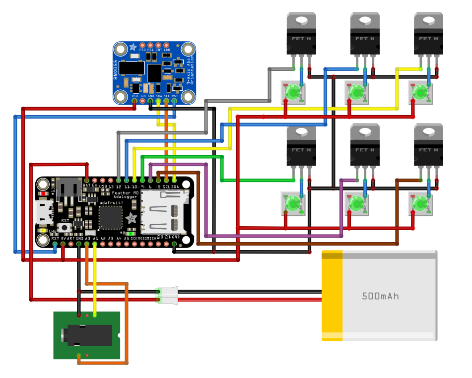
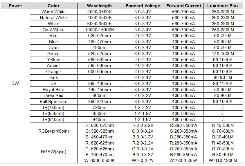
The main components include a microcontroller, LiPo battery, and LEDs. I selected the Adafruit Feather M0 Adalogger for the microcontroller. It has a very small form factor, has many IO pins, and requires only 3V power. I was already familiar with the microcontroller as it can be programmed like an Arduino and I had already used in for the FDR. I also selected the same lights as on the BL-NavLV, 3W LEDs. They are well suited for the application because of their brightness and low power requirement. A 3W LED can produce over 100 lumens, which is visible for at least 400 ft in the daytime.
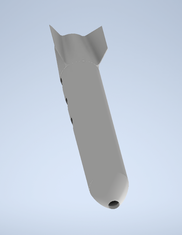
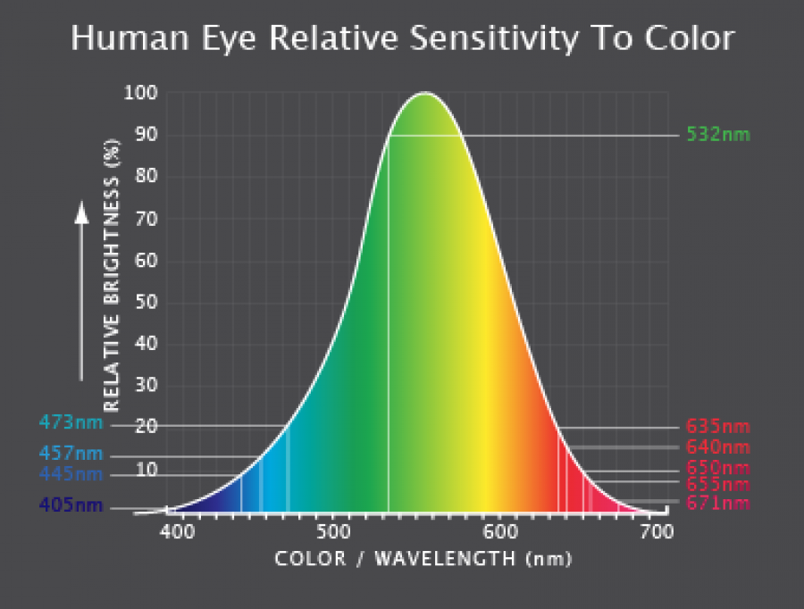
The sensor has 6 LEDs oriented in columns of three. The diodes have a wide 180 degree viewing angle. This allows at least 3 LEDs to be visible from a side on view. The optimal color of the LEDs is green, since the biology of the human eye is most attuned to the wavelength of green light. Green also contrasts well to the blue sky, as opposed to white. Each green LED can provide 160 lumens at a maximum rated 500 mA draw. Each LED is visible for at least 400 ft during the daytime.
Powering an LED is a tricky business. They are very sensitive to current, and too much current can burn them out, making them unusable. Therefore, many LEDs are driven by constant current supplies. One option is to use a boost/buck converter. These act as a regulator between the LEDs and the battery. However, one of those converters typically require an overhead of 3V, which means I need 3V for the LED + 3V for the dropdown = 6V LiPo battery. Such a battery is would not meet the size constraints.
A simpler option is to overdrive the LED and remove the regulator all together. The LEDs could be connected directly to a 3V power source, and with the right current capacity, the LEDs could be powered at their maximum brightness. The problem was that the LEDs had to be connected to the digital pins on the Feather so they could be flashed in a programmable pattern. Each digital pin can output at most 10 mA while the LEDs require at least 500mA, a order more of current. This necessitated a MOSFET for each LED, connected to the microcontroller between each LED and the battery. IRFZ44N MOSFETs were selected because of their low gate threshold voltage which is suitable for the 3V logic of the microcontroller. The MOSFET allow unrestricted flow from the battery to the LED when switched on by the digital pin of the Feather.
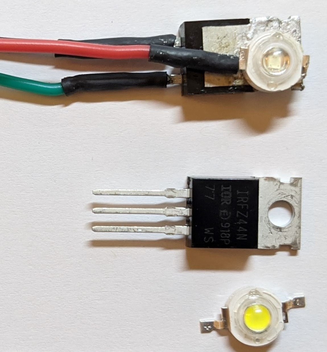
The LEDs were soldered to the MOSFET heatsinks to prevent overheating and diminishing brightness over time. The large heatsink on the MOSFET is operating well below its maximum rated capacity. So, it could also be used to cool the LED if they are in contact. The back of the LED has an isolated metal plate, while the heatsink conducts to the drain. Soldering these two surfaces together provides good thermal conductivity and does not affect the circuitry. It would even make the circuit more compact, as a wire is saved by connecting the cathode of the LED to the heatsink.
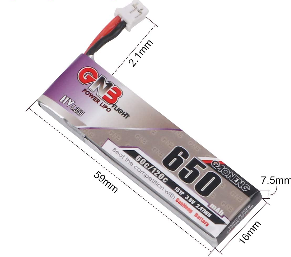
The battery selected is a 650 mAh 60C 3.4V LiPo battery. The rechargeable nature of LiPo batteries and their high power density make them an optimal choice. It can supply 13 min of runtime with all LEDs running simultaneously at a total 3A current draw. More likely, the battery could last over an hour with each LED blinking individually. The 60C rating is also more than sufficient for this application. Battery calculations are shown below. \(\begin{align*} \text{Runtime at Max Current Draw:}\\ C &= I_{draw} * t_{runtime} \\ 650 &= (6 LED * 500 mA/LED) * t_{runtime}\\ t_{runtime} &= 0.217 \text{ hours} \\ &= 13 \text{ minutes} \\ \text{Maximum current draw:}\\ I_{max} &= \frac{C}{1000} * C_{rating}\\ I_{max} &= \frac{650}{1000} * 60\\ I_{max} &= 39A \end{align*}\)
CAD Design
Early Prototype
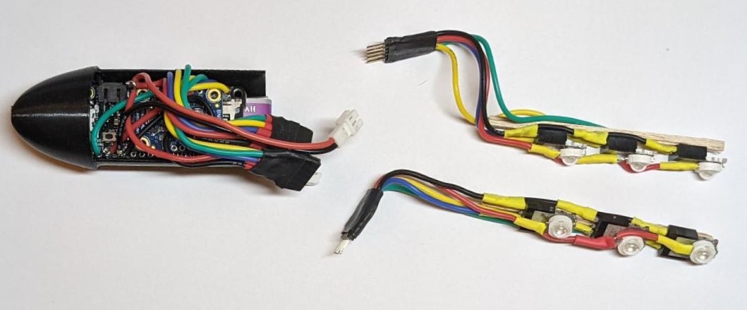
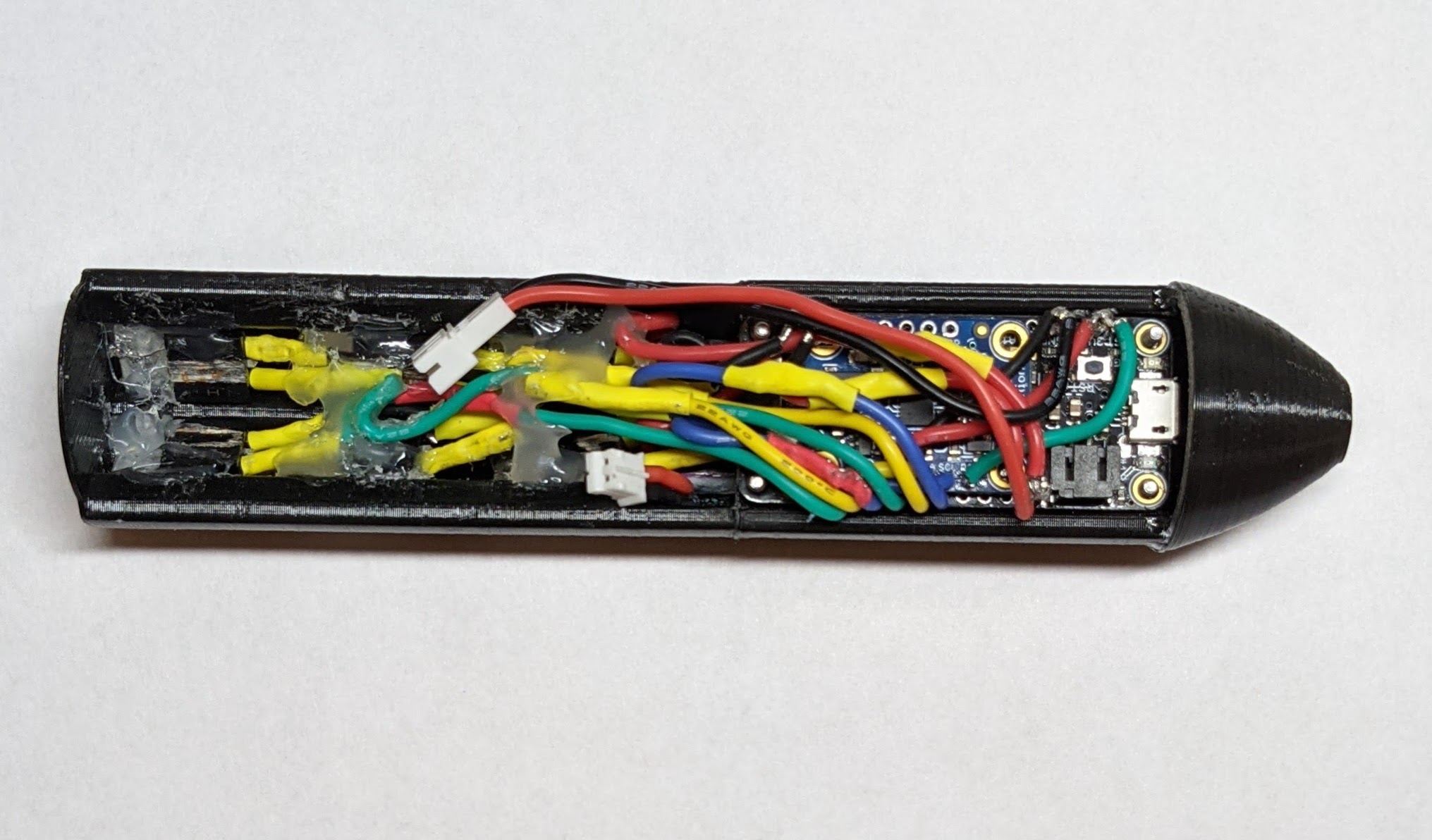
As the electronics started coming together, it became clear that the space in the sensor would be very limited, and the electronics would need to be arranged as compactly as possible. The sensor housing would also need to allow easy access to the electronics to make alterations and to recharge the battery. I decided to make a two-part assembly. There would be the nose cone assembly and the sleeve. For the first prototype, I decided that the nose cone assembly would hold the battery and the microcontroller in a semi-circular tray. It would be able to slide in and out of the sleeve, which housed the LEDs. The LEDs would connect to the controller using two 5-pin connectors made from male-female header strips. The purpose of these connections was to allow the LEDs to detach from the controller so the assembly pieces could be swapped out. Several sleeve designs were be experimented with, and they could all adapt to the same nose cone thanks to the modular design.
Final Design
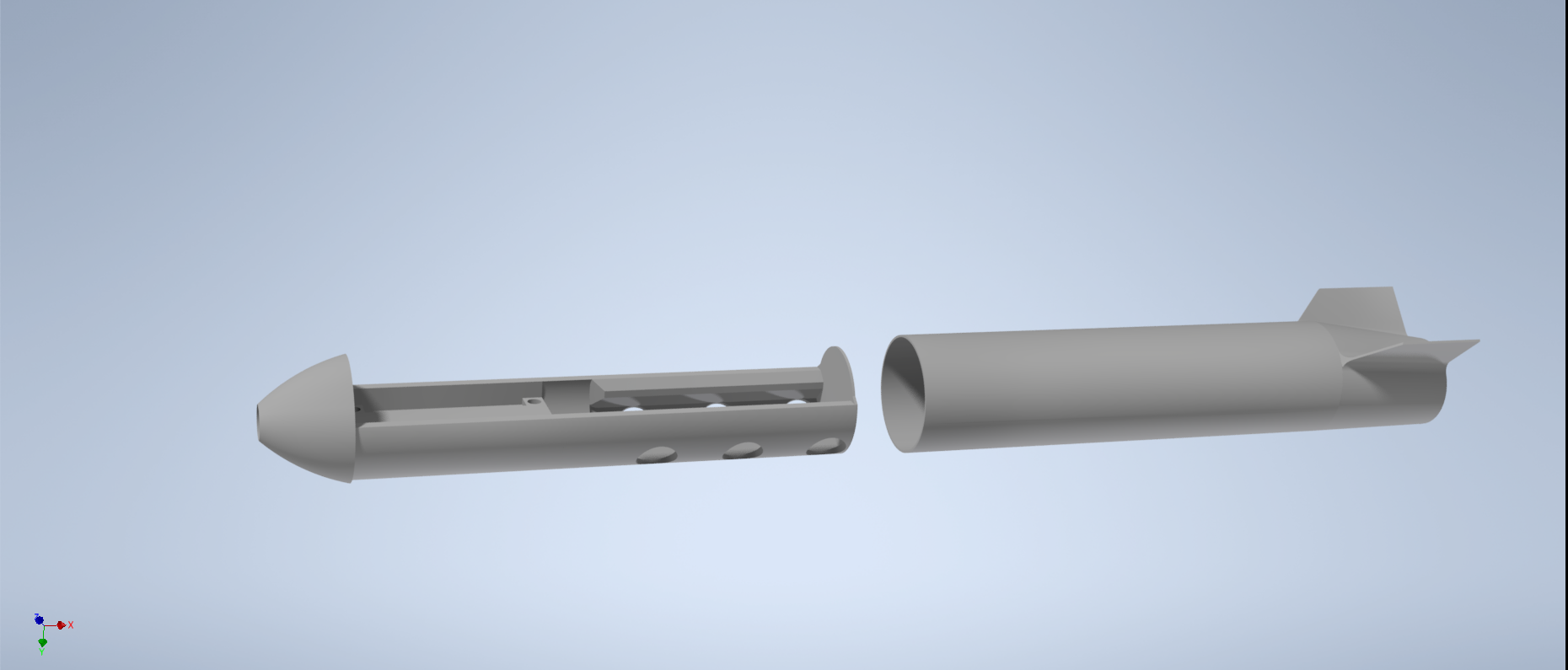
There was a big difference between the early prototype and the final design. Most notably, the CAD design was a more detailed, with secure mounting points for all of the electronic components. The electronics tray was also extended to include the LEDs and the connectors were removed. This made the sleeve easier to remove and swap out.
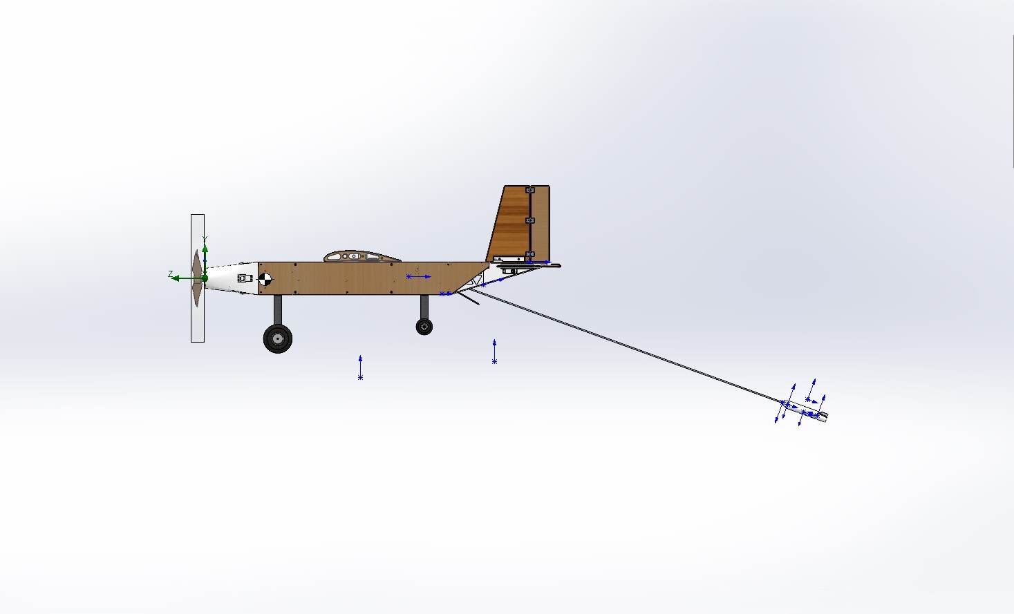
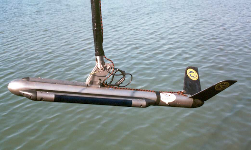
The sensor consists of four 3D printed parts: the nose cone, controller housing, lighting assembly, and outer sleeve. While each part is printed separately, the nose cone, controller housing, and lighting assembly are glued together to form the electronics tray. This tray secures all the electronics including the battery, controller, and LEDs. It also interfaces with the tow cable through a hole in the nose cone. The outer sleeve is interchangeable, and slides firmly over the tray. It is locked to the tray assembly with a single screw through an alignment hole. This allows for easy access to the electronics. The sensor weighs 0.206 lbs, with the bulk of the mass concentrated at the lower front of the sensor. This design decision provides inherent stability as the center of gravity is located in front of the center of pressure.
Controls Implementation
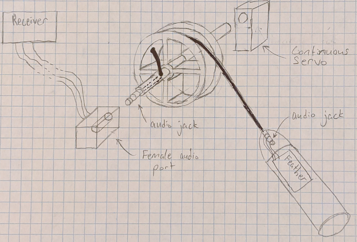
The sensor is controlled from the ground via the transmitter. An extra channel on the remote is used to send an “on” signal to the receiver. The signal is picked up by the receiver and is transmitted as a PWM signal through the tow cable to the sensor. The sensor’s built in microcontroller detects the input signal and begins a lighting sequence. Each LED is programmed to flash one at a time in a repeating pattern. An audio cable was selected as the tow cable to transmit the signal, as it is multi-wired and allows for 360 degrees of rotation. Two of the channels were utilized – ground and signal. The end of the audio cable attached to the winch formed the axle, which allowed a signal to be transmitted no matter the angle of the winch.
Performance Testing
Sensor flight tests were conducted during December 2020 and January 2021 to determine the performance of the various sensor designs over a range of air speeds. The sensor collects data from its onboard IMU to a microSD card in CSV format. The data collected includes 9-axis absolute orientation, angular velocity, and linear acceleration data. This data is analyzed and used to to determine flight characteristics and finalize stabilizer fin shape. Other metrics can be estimated including average tow cable angle and standard deviation. The testing procedure is detailed below.
Test Setup
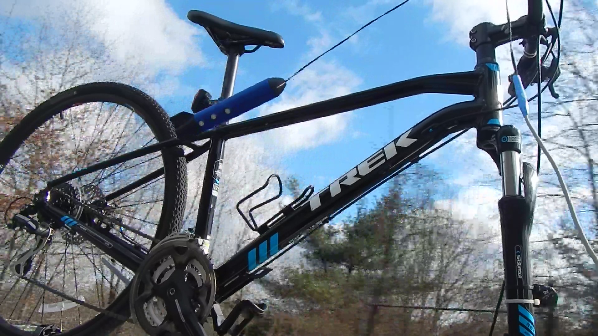

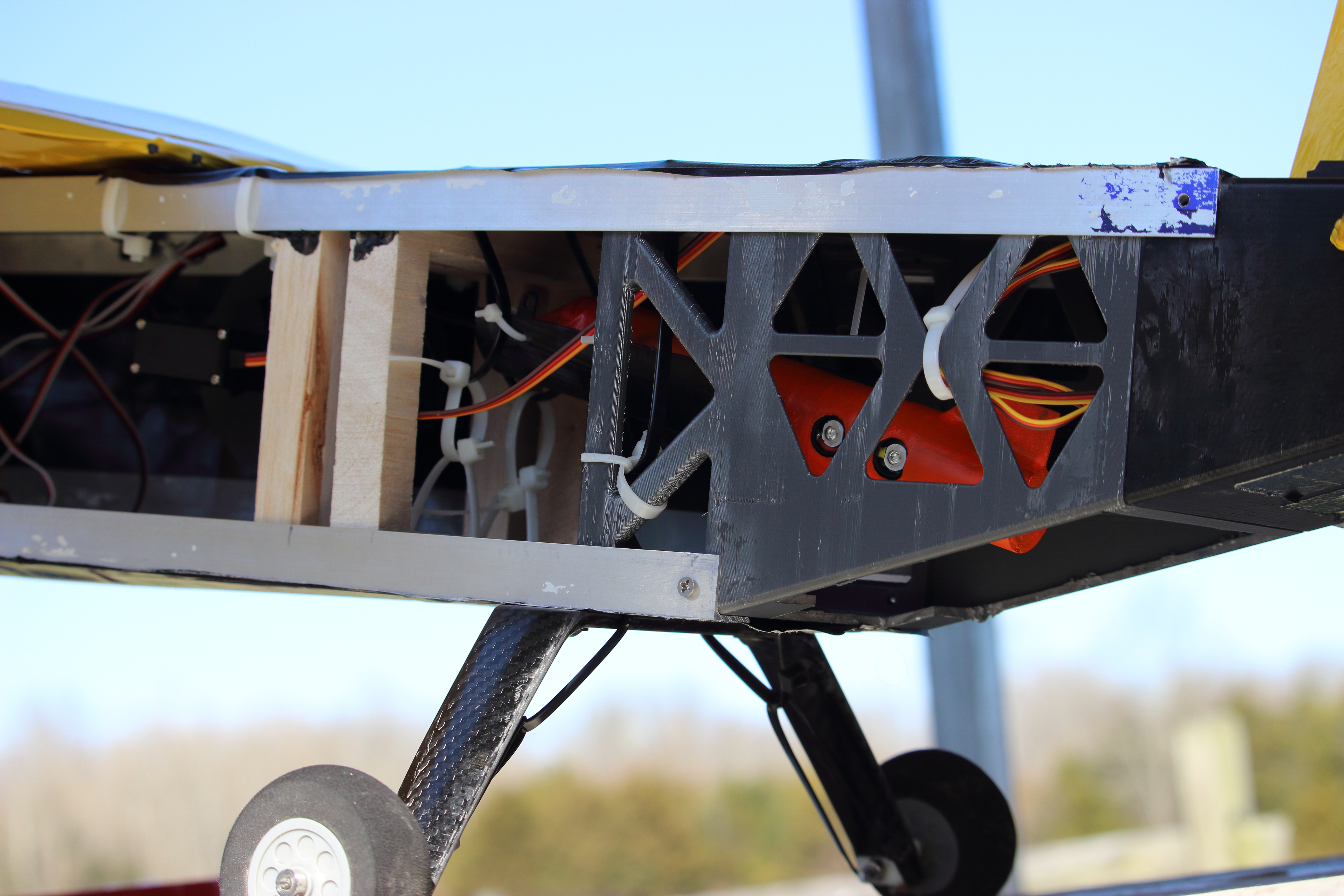
The sensor was mounted to a bike on the roof of a car as seen in Figure X. The audio tow cable was attached to the bike handlebar to keep the sensor above turbulent airflow coming over the car. The test route was a straight stretch of road, seen in Figure X. Each sensor design was tested in intervals from 30-60 mph. For each test, the car would accelerate to the testing speed and proceed to cruise at a constant speed for the duration of the test. A Flight Data Recorder mounted in the car initiated sensor data recording via a control signal through the audio cable. The FDR was also used to collect baseline data including GPS coordinates, heading, and speed. The data results were analyzed using Python and are summarized in the Results section.
Performance Results
Test Results
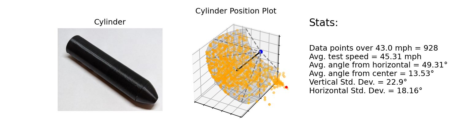
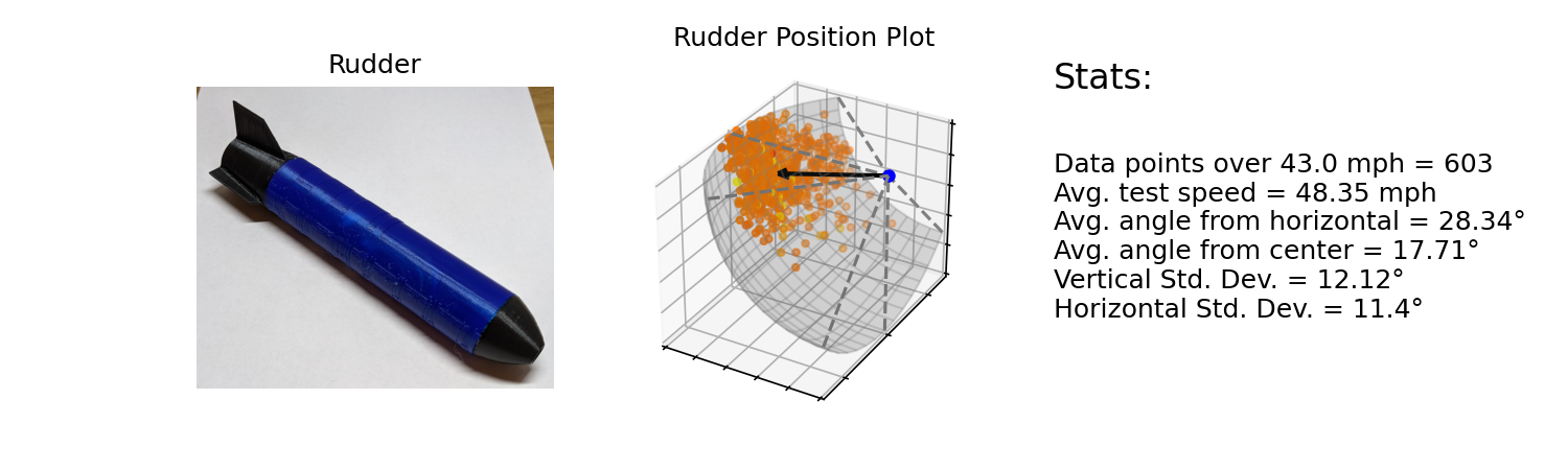
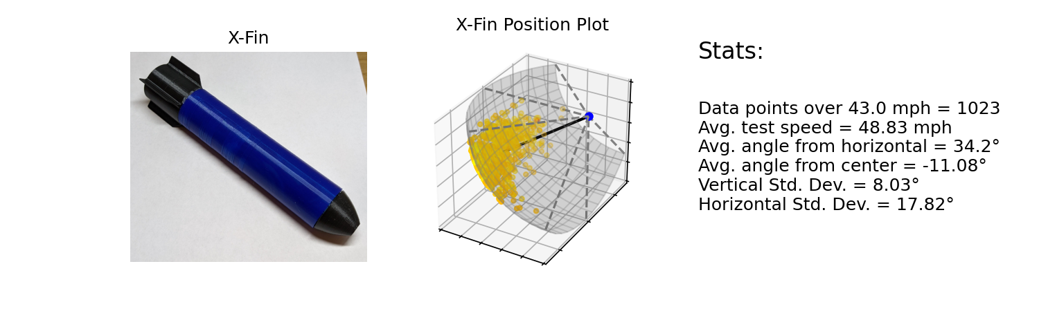
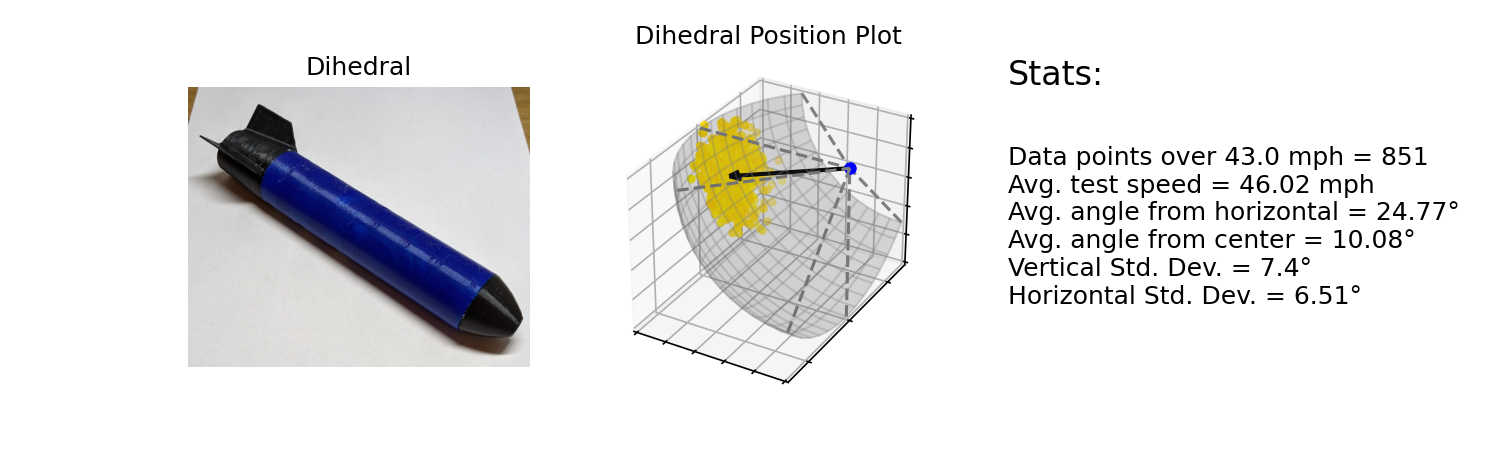
Sensor aerodynamic behavior was captured via an onboard 9-axis IMU. The data was plotted onto a position scatter plot, showing the positions of the sensor relative to the car’s inertial reference frame. Figures X-Z below show the average angle of inclination and standard deviation of each sensor design. The lower the standard deviation of the tow cable angle, the more stable the sensor was. These statistics give the team quantitative measurements to aid in the final selection of the sensor design. While the dihedral design was already determined to be the most promising design, these results confirm the team’s findings. The dihedral design had the best performance of the bunch, with the lowest variance in tow cable angle. It also maintained the lowest angle from the vertical. The other sensors struggled to maintain a consistent heading, and were not stable designs.
Additionally, the testing results can be used to verify initial drag estimates. The experimental data is analyzed to determine the sensor’s actual coefficient of drag. Comparing the actual coefficient of drag to the estimated coefficient of drag can provide information on the quality of the estimations made. The analysis was conducted on the test with the most calibrated data points at 70 ft/s and 34° from horizontal. The team measured \(C_{D, actual} = 0.293\). The sensor’s actual coefficient of drag has a 9.29% error from the estimated \(C_{D, est} = 0.323\). This percent error is deemed acceptable given the variability of doing a real world test.
\[\begin{align*} \text{Equations:}\\ C_D&=\frac{2D}{\rho V ^2 A} &\text{Equation 1: Coefficient of Drag}\\ C_l&=2\pi \alpha &\text{Equation 2: Thin Airfoil Theory}\\ F_L&=\frac{1}{2}C_l \rho V^2 A &\text{Equation 3: Modern Lift Equation}\\ F_b &= \rho g V &\text{Equation 4: Buoyancy Force}\\ \text{Constants:}\\ A&=\pi r^2=0.000792 m^2\\ V&=\pi r^2h=0.00015 m^3\\ m&=0.0934 kg\\ \alpha & =0.5969 rad\\ v&=21.82978 m/s\\ g&=9.81 m/s^2\\ \rho &=1.225 kg/m^3\\ \text{Calculations:}\\ F_d &= \frac{F_g-F_L-F_b}{tan(\alpha)} &\text{From Free Body Diagram}\\ &= \frac{mg-\pi \alpha \rho v^2A -\rho gV}{tan(\alpha)}\\ &= 0.07084 N\\ C_d&=\frac{2F_d}{\rho v^2A}\\ &=0.293\\ &\frac{0.323-0.293}{0.323}*100 \% =9.29 \% &\text{ Percent Error}&\\ \end{align*}\]Stabilizer Fin Decision Matrix
| Criteria | Weight | Cylinder | Large Rudder | X fins | Dihedral |
|---|---|---|---|---|---|
| Stability | 65% | 1 | 3 | 4 | 5 |
| Storage Density | 25% | 5 | 2 | 3 | 4 |
| Drag (low) | 10% | 5 | 4 | 3 | 1 |
| Weighted Score | 2.4 | 2.85 | 3.65 | 4.35 |
The weighted decision matrix for sensor fin design is shown above, with the dihedral fin selected as the final design. The control cylinder had low drag and a high storage density for the cargo mission, but without fins it had poor aerodynamic stability. The large rudder fin design helped keep the sensor in an upright flight orientation, but it chaotically fluttered on the tow cable. The X-Fin’s symmetric shape had significantly more stability than the previous options with moderate storage density and drag. The dihedral fin design best maintained an upright attitude and stability during testing, likely due to the dihedral effect. It also had a higher cargo storage density.
Flight Results
The final sensor performance exceeded our expectations. The special mission component underwent consistent and reliable deployment and retrieval operations. The sensor was aerodynamically stable with no fluttering or adverse affect on aircraft controllability. The sensor also proved itself in endurance testing, flying for a 10 minutes with sensor lights visible from the ground.
The aircraft was also amazing. It flew gracefully with more than sufficient maneuverability, power, and predictability. As per our test pilot Tony, “It flew like a kitten.” It was quite an accomplishment for the entire team and we were ecstatic to say the least.
What I Learned
It was also a unique experience for me to work on a team of primarily mechanical, aerospace, and systems engineers. I learned a lot of new skills. One lesson was the value of communicating design methodology and interfaces with various subteams. I also learned the hard way of the importance of using modular and interchangeable designs. It makes testing and experimentation a lot easier. Last but not least, I learned how to write a formal design report and effectively convey design decisions.
I was originally drawn to the UAV Towed Sensor because of the blend of hardware and electronics design. But, I also saw the potential to make a smarter sensor by incorporating a microcontroller and IMU. I love using low cost, unobtrusive sensors because they can provide critical insights on current design performance which translates to a better design in the next iteration and so on. The UAV Towed Sensor was also a natural extension of Flight Data Recorder project. I was able to incorporate some of the same hardware, software, and data analysis.
The success of both these projects inspire me to continue developing computing projects that sense and interact with the physical world. I hope to continue developing the FDR and working on aircraft flight computers. The use cases for these sensors are also endless, with practical applications in wearable technology and robotics. I hope to tinker in some of these directions as well.